Analyzing by Learning Samples
Dimensionality reduction is a function to “compress” multi-dimensional cell data to display it on a two-dimensional plot by applying the technology of machine learning. You can use either the “UMAP” or “FIt-SNE” dimensionality reduction technique.
Set the learning conditions, and analyze by learning samples. With dimensionality reduction, you can select a density plot or dot plot.
- Select the gates to be analyzed, and click [UMAP] or [FIt-SNE] in [Dimensionality Reduction] on the [Gate] tab of the ribbon.
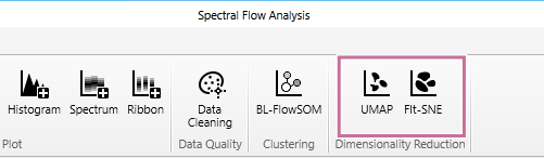
The [UMAP] dialog or [FIt-SNE] dialog appears.
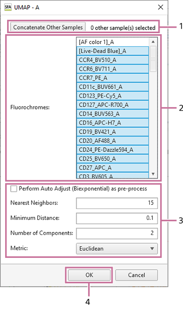
- Set each item, then click [OK].
When [UMAP] is selected
When [FIt-SNE] is selected
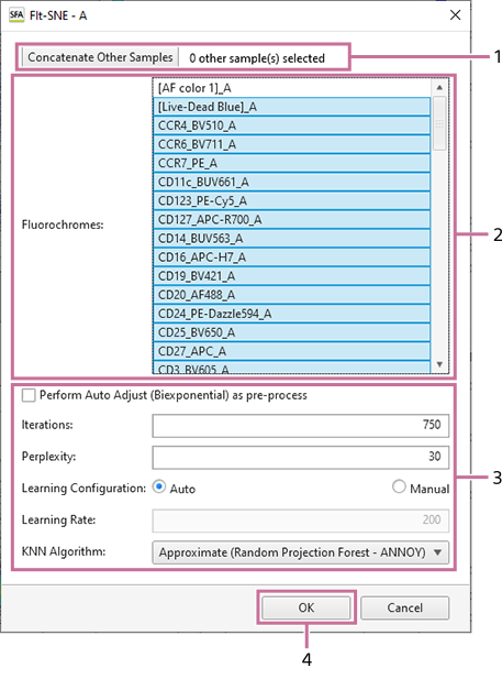
- Select the samples to concatenate when analyzing by concatenating samples.
For details about the operation, see “Analyzing by Concatenating Multiple Samples (when UMAP and FIt-SNE).”
- Select the fluorochromes to use as inputs.
- Configure the learning parameters.
- Click [OK].
- For details about each setting item, see “[UMAP] Dialog” and “[FIt-SNE] Dialog.”
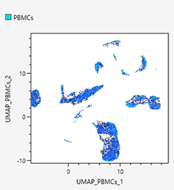
An empty plot is displayed during learning. When leaning finishes, a density plot for the learning results is displayed.
- Select the samples to concatenate when analyzing by concatenating samples.
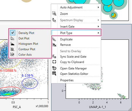
- Select the plot type, as required.
Right-click within a plot, select [Plot Type] in the context menu, and select the plot type.
Select any of [Density Plot], [Dot Plot], [Histogram Plot], [Contour Plot], and [Color Axis] for the plot type.
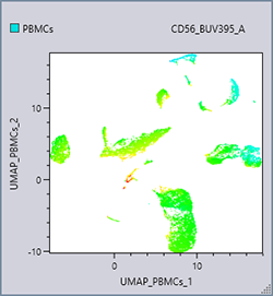
A color axis displays the specified fluorochrome emphasized. It is suitable for viewing the expression intensity. Using a color axis in combination with dimensional compression can be useful.
- With a dot plot, you can color specific cell populations. For details about the operation, see “Coloring Cell Populations (Dot Plot).”